
|
SpinalTap
/ 502 Project |
| Overview |
| SpinalTap
was a virtual surgery project that came about because Marilyn Powers (a
Mechanical Engineering PhD student) needed a program that used the haptic
(force-feedback) drill she was designing. The program she had in mind was
a training simulator that surgeons could (theoretically) use to practice
spinal drilling procedures. This stuff is really dangerous and practice
is hard to come by. So we set out to build a virtual surgery system starting
in September 2001.
Fast-forward to April 2002, when I realized that there was no way I was going to finish an entire surgery simulator. So a massive reduction in scale took place, and I was left with SpinalTap: An Architecture for Real-Time Vertebrae Drilling Simulation (also available in Postscript, with nice pictures). The Powerpoint slides for the presentation I gave to my comittee are also available.
|
| SPINAL SURGERY !?!??! |
|
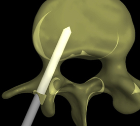
Yea, spinal surgery. Specifically, pedicle screw insertion. The surgeon drills a hole and inserts a pedicle screw to stabilize two vertebrae during the fusion process (that's what they do after you rupture a disc in your spine). The images below should give you an idea of what actually takes place.
|
| A Virtual Vertebrae |
| The
problem with virtual spinal surgery is that you need a virtual spine. The
naive approach is to whip out Maya and make one. One problem with that plan
- the system has to be realistic. Realistic as in the density feedback from
collision detection has to be relatively similar to real bone. Real bone
is tricky, especially when there are areas affected by osteoperosis. Osteoperotic
bone is really brittle and the drill cuts through it like butter (that's
why the surgeons need to practice). The only way to get accurate bone density
data is to use a real-world data source - CT scan slices.
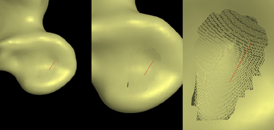
You can see a vertebrae CT slice in the left image below. CT slices are generally distributed in sets, the whole set is called a stack, and it gives you the vertebrae volume at a relatively low voxel resolution. The slice below is taken directly from the CT stack - no scaling. That's not a lot of pixels. The middle image shows just how noisy this data really is, and the right shows a segmented slice (why is it segmented? keep reading).
We also needed a point inside-outside test for the collision detection scheme, so an implicit surface was the obvious way to go. Normally fitting an implicit to arbitrary data (like CT scan data) is really hard. Luckily, there is this nifty Radial Basis Function (RBF) technique that was presented at SIGGRAPH 2001, and FarField Technology has a trial version of their 3D Fast Multipole Method RBF fitting software. All I needed now was a set of surface points. The basic idea was to isolate a stack of contours from the CT slices. By 'stack of contours' I mean the set of surface pixels in each slice. Doing this properly was difficult because a) I'm not an expert and b) I didn't have any tools or software designed for this process. In retrospect, I should have found some. What actually happened was that I manually segmented the CT slices. That took a while. Then I smoothed the edges out by hand because they were too rough. That took even longer. The final point set I isolated is show below left, and the final RBF is on the right. Click for bigger images.
|
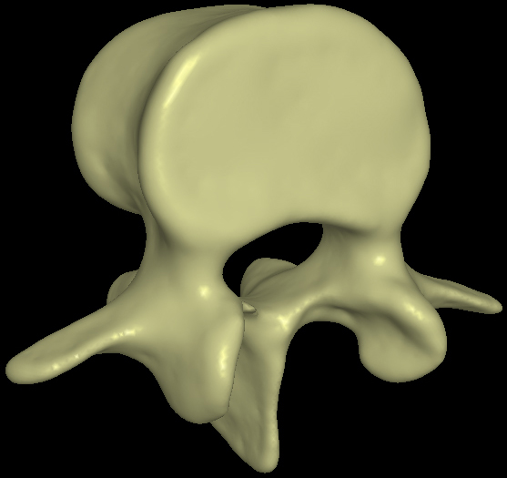
| Fitting the Vertebrae Surface |
|
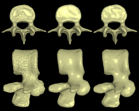
Creating a smooth implicit surface for the vertebrae turned out to be a rather difficult problem. The RBF fitting process guarantees that the output surface will smoothly interpolate the set of points you give it. It works best when your data distribution is relatively uniform. Our distribution was not relatively uniform. You might notice in the point set image above that there are some rather large holes - specifically on the front and back faces of the vertebrae lobe. This is due to the CT data. These ugly areas, along with some alignment problems between slices, resulted in a very rough surface (below left).
A relaxation or smoothing factor can be added to the RBF fitting process. This allows the surface to not exactly interpolate the points you give it. I cranked up the smoothing and got the surface on the right. That surface looked pretty good, but it had a small problem. When you add smoothing you permit volume change. The smoothed surface on the right had a lot of volume change. The image below shows the silhouette of the unsmoothed surface (red) superimposed over the smoothed surface (white). The volume inside the white areas does not exist in the CT data, hence the bone density there is zero. This is obviously a bad thing. (The big number is the smoothing factor. The above right surface has smoothing = 30 ).
I thought the real surface was too rough and the smoothed surface was wrong. I was in a bit of a bind. Luckily, there is another way to smooth the surface - increasing the off-surface point distance. Read my report or find an RBF paper to find out more. The result of this modified fitting process was the middle surface. It lacks the major volume change but it's still smoother. One small note here. When I looked at the initial really-bumpy vertebrae,
I figured it was all wrong. I kept hacking at it until I got the really
smooth version. Then I presented it to my comittee and found out that
vertebrae aren't really that smooth. Oops. Moral of the story: always
ask an expert. |
| Collision Detection |
| Now
that I had a virtual vertebrae, I needed to destroy it. The drill volume
was represented by a cylinder with a conical end-cap. I also had another
handy bit of info: surgeons plan out in advance where they are going to
drill (and they stick to it). Collision detection also needed to be really
fast. At least 100Hz, and possibly over 1000Hz. Oh, and it needed to be
really accurate.
The algorithm I came up with involved point tests. Basically I created a cylindrical point volume where points were distributed around rings in discs in the volume, all at 0.1mm intervals. Hopefully the picture below will explain what I mean. The point volume I used for most of my tests had 986,958 points.
By exploiting the geometry of the drill, I could do some very efficient culling of the points that needed to be tested for collision It is guaranteed that any inner ring must be fully destroyed before the next outer ring can be fully destroyed, and once a ring is fully destroyed it does not have to be tested. We can also calculate the furthest possible outside ring that could be intersected in any given disc. The naive algorithm I implemented has one rather important flaw - it strongly favors on-path drilling. The 'path' is the vector down the center of the point volume cylinder (it goes through the center of each disc). As the drill strays off the path, more rings need to be tested each frame. This situation is illustrated in the image below. Testing all these extra rings causes a significat slowdown. However, a modification to the algorithm is possible that will fix this problem. Since the drill is convex, it will only intersect each ring in at most two places. This means we can start in the middle of the collision interval and walk in both directions around the ring. Once we hit the surface in each direction (or cross over), we are done.
One small problem was left. After the surgeon drills the hole, he might want to look at it. The vertebrae surface was rendered as a triangle mesh and updating this mesh was not an option. I decided to use a simplified splatting technique to render the area around the drill hole. During the point volume generation process I cut a hole in the mesh. While the simulation was in progress I simply rendered all the discs marked as surface discs. The results of this splatting process are shown below. A problem here is that as you zoom in, the surface breaks apart. More complicated splatting algorithms can deal with this problem.
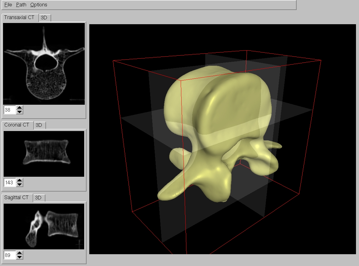
One last picture before the results. This image is cut from a screenshot of the drilling simulation in action. The vertebrae surface is rendered transparently, so you can see the set of surface discs being rendered, along with the drill model. The path shown is similar to the actual path used for pedicle screw insertion.
I wrote a small simulator to test the performance of the collision detection algorithm. The graph below shows four runs of the simulation. Collision detection frequency is plotted on the vertical axis and distance along the drill path is on the horizontal axis. The two higher graphs are on a dual PIV/1400 Mhz machine, the lower two are on a dual PIII/733 Mhz machine. In each pair, the (generally) slower simulation was set to be off-path, showing that the algorithm is indeed slower in this case. The speed drops as you drill along the path because more points have to be tested. See the paper for an in-depth analysis, including an explanation of the Pentium 4's erratic behaviour. (Click the image for version where you can read the captions).
As you can see, I hit my design minimum of 100Hz. The PIV was over 400Hz.
One important note was that the collision detection algorithm only ran
in one thread. The algorithm should scale close to linearly with processor
count. Spreading the detection load over multiple processors (say a quad
Xeon machine) should give us detection rates well over 1000Hz. |
| Conclusion and Parting Shots |
| The
project was deemed a success by the comittee, although I don't feel that
I got far enough (always the perfectionist). I was not terribly motivated
to fix some of the problems I encountered because I didn't have a big interest
in the final system. The user interface for the path planner was particularly
unimpressive IMO (although Lars thought the transparent guide planes were
great). Here is a screenshot.
I'm basically finished with SpinalTap. However, several professors in
the Computer Graphics and Mechanical Engineering departments at the University
of Calgary have an interest in seeing this project move forward. If you
are interested, mail me or
blob. |
|
Questions?Comments?
Email rms@unknownroad.com. |